1. Introduction
Modern IT companies operate in conditions of high external dynamics, constant technological changes, and the need for rapid adaptation of business processes. Under these conditions, the effectiveness of teams becomes particularly significant, as the main organizational unit responsible for implementing digital products and services. At the same time, traditional approaches to assessing work results, based on individual indicators or linear KPIs, turn out to be insufficient for a comprehensive evaluation of a team’s contribution to achieving the strategic goals of an organization [1].
The relevance of the research is driven by the need to develop a systematic and flexible approach to forming team effectiveness metrics that take into account the specifics of IT activity, Agile methodology, and project culture. Practice shows that even transparent and evidence-based performance indicators often face difficulties in managing productivity, motivation, and staff development [2].
The goal of this study is to develop a methodological approach to constructing a system of team effectiveness metrics in IT companies. To achieve this goal, the article considers existing models for performance assessment, analyzes their applicability in the context of digital organizations, and proposes a conceptual framework for structuring indicators along three directions: result-oriented, process-oriented, and behavioral.
The novelty of the proposed approach lies in clarifying the principles for forming team effectiveness metrics with consideration of the cyclical nature of product development and the interaction of cross-functional groups. The practical significance of the study consists of the possibility of using the proposed approach when building analytics and management dashboards in IT organizations.
2. Review of Existing Approaches to Assessing Team Effectiveness
The problem of measuring team effectiveness in work and organizational literature is considered from different perspectives. Traditionally, three approaches are distinguished: result-oriented, process-oriented, and behavioral [3]. The result-oriented approach focuses on assessing whether target indicators (KPI, OKR) have been achieved, providing a connection between team activities and the strategic goals of the organization. However, this approach often ignores the quality of internal team interactions and the specifics of the development process, which is particularly critical for IT projects [4].
The process-oriented approach focuses on studying the parameters of production flow and internal processes that influence the final result. Within flexible management methodologies, primarily Kanban and Scrum, team effectiveness is assessed not only by final results, but also by the stability, predictability, and uniformity of production flow. In this case, the key metrics are cycle time (task completion time), lead time (time from request to delivery), throughput, and WIP (work in progress) volume [5]. These indicators allow managing team workload, identifying bottlenecks, and increasing transparency of the development process.
Supporters of the behavioral approach emphasize the importance of non-material factors: trust, autonomy, and engagement [6, 7]. For IT teams working in a cross-functional environment, these parameters are often linked to adaptability and decision-making speed. Nevertheless, behavioral aspects are difficult for quantitative measurement and require a combination of qualitative and quantitative methods.
Thus, the analysis of existing models shows that traditional KPI and OKR approaches do not provide sufficient flexibility. Agile methods, especially Kanban, offer tools for continuous flow analysis and adaptive performance management. This determines the need to form an integrated methodological approach that combines Kanban transparency principles with the strategic orientation of classical management models.
3. Methodological Foundations for Developing Team Effectiveness Metrics in IT Companies
3.1. General Principles
The proposed methodological approach is based on the principles of flow management and continuous improvement underlying the Kanban method [5, 8]. The focus is on managing the time of task progression (lead time) and statistical behavior of the process. This approach allows considering the team as a service system with predictable flow characteristics, where result-oriented indicators reflect the stability of value delivery to the customer.
Unlike traditional KPI models, where analysis is limited to final indicators, Kanban focuses on transparency of processes and work with sources of variability in the system. The key idea lies in controlling flow indicators and understanding the behavioral patterns of the system based on data.
3.2. Logic of Analysis: from Lead Time to Flow Structure
The core of the proposed methodological approach is the stage-by-stage analysis of the delivery process using flow metrics. The first step is the analysis of the overall lead time, which reflects the total time a task spends from the moment it enters the system to its completion. The median value and the 85th percentile are calculated, which make it possible to assess the predictability of the process and the service level.
Next, the lead time is decomposed into stages: discovery, decomposition, development, and A/B testing. This allows identifying the stages that have the greatest impact on the duration of the cycle and defining the “bottlenecks” of the process.
The next stage is the analysis of dynamic indicators by quarters, aimed at evaluating the impact of managerial decisions (for example, introducing WIP limits or changing readiness criteria) on cycle stability.
To visualize the flow stability, a cumulative flow diagram (CFD) is used, showing the balance between incoming, in-progress, and completed tasks. The presence of “bands” in the diagram signals fluctuations or overloads in the team’s workflow.
The final stage is a detailed analysis of outliers beyond the 85th percentile. This step makes it possible to identify the reasons for deviations (unclear requirements, repeated returns, priority violations) and formulate corrective managerial decisions. Together, these stages form a complete methodological process analysis system, where the focus is placed on maintaining flow predictability.
4. Practical Section: Applying the Methodological Approach in the IT Company hh.ru
4.1. Organizational Context of the Study
The analysis is conducted using the example of a product team at hh.ru, which operates according to the Kanban methodology and is responsible for the development of one of the company’s internal services. The team is characterized by high autonomy, a cross-functional composition, and a continuous flow of tasks formed by user requests and the needs of related departments. The main goal of the analytical work is to improve the predictability of delivery timelines and reduce the response time to changes in requirements.
4.2. Stages of Analysis
The application of the methodological approach includes several key stages.
Analysis of Overall Lead Time. At the first stage, the median lead time and the 85th percentile of the distribution of task completion time are calculated for the quarter. The use of the 85th percentile is explained by the fact that this metric reflects realistic expectations of delivery considering the natural variability of the process without distorting the data with rare outliers. Thus, the 85th percentile serves as the Service Level Expectation (SLE), allowing managers to plan deadlines with a high probability of compliance.
On the chart of lead time (Figure 1), a clearly pronounced peak in the 50 to 60 day range is observed, and the short tail of the distribution indicates the stability of the process and its uniformity. The absence of a long tail suggests that the team does not experience significant deviations in task execution: extremely long tasks, which could distort overall statistics, are almost absent.
The pronounced peak in the middle of the distribution means that most tasks are completed in approximately the same amount of time. This characterizes the team as predictable, with stable throughput, and enables the use of the 85th percentile as a planning tool.
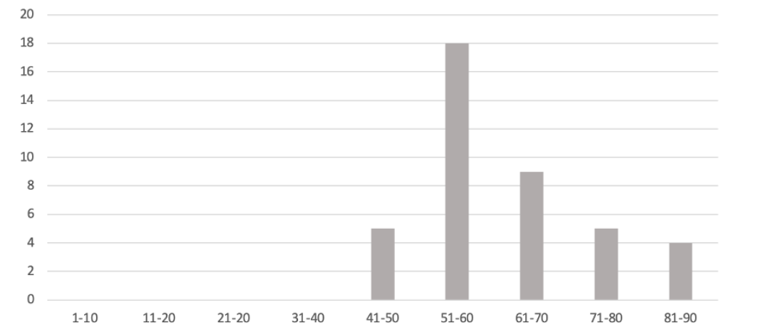
Nevertheless, the peak itself carries additional analytical value. The presence of a distinct peak reflects the dominant service class: the type of tasks that forms the main flow. In this case, judging by the average lead time, these may be standard product enhancements that pass through the full cycle “discovery → decomposition → development → testing”. If the distribution contained several peaks, this would indicate a mixture of different task classes, for example, short technical fixes and long research-oriented projects. In such a situation, the flow analysis would require separating tasks into categories to more accurately forecast delivery times for each type of work.
It is also important to note that the absence of a long tail does not always guarantee an ideal process. In some cases, this may indicate strict filtering of tasks or an underestimation of complexity during intake, when “non-standard” tasks simply do not enter the flow. Therefore, when interpreting the histogram, it is useful to compare it with other visualizations, such as stability control charts and cumulative flow diagrams (CFD), which help confirm the stability of the production rhythm.
Overall, the chart demonstrates that the team has achieved a predictable and controllable delivery cycle, without outliers. This allows lead time to be used not only as a control metric but also as the basis for forming SLA and forecasting team workload for the next quarter.
Decomposition and identification of bottlenecks. Lead time reflects the high-level state of the system, but to understand which factors influence the duration of the cycle, it is necessary to examine its component stages. For this, the distribution of time across stages is analyzed: discovery, decomposition, development, and A/B testing. Such analysis makes it possible to determine which stages have the greatest impact on the overall cycle duration and where the primary reserves for improvement are concentrated.
Figure 2 shows box plots by stage, where for each stage the 1st, 25th, 50th, 75th, and 100th percentiles are displayed. The closer these values are to one another, the more stable and predictable the process is. A narrow gap between the median and the upper quartile indicates that the task execution time at that stage changes only slightly, and the team effectively controls the flow. Conversely, a large gap between percentiles indicates high variability: some tasks pass quickly, while others take significantly longer, which reduces the predictability of the entire value chain.
The chart shows that the “Development” stage has the widest spread of values and the highest 85th percentile, which makes it the primary candidate for optimization. Long and unpredictable development cycles may be associated with insufficient Discovery of requirements, overload of developers, or accumulation of technical debt. The “Decomposition” and “Discovery” stages, by contrast, are characterized by narrower ranges of values, which indicates stability and controllability at these steps.
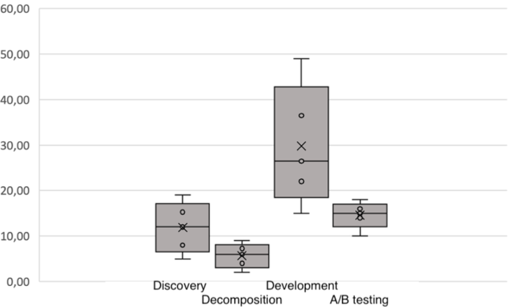
An interesting direction for improvement may be increasing the quality of decomposition. If, at the stage of decomposition, tasks are broken down insufficiently deeply, part of the uncertainty transfers into development, increasing both the duration and the variability of the cycle. More detailed decomposition and clarification of readiness criteria before development can reduce the range of time values, decrease the share of long tasks and, consequently, reduce the overall lead time. It is important to note that this is only a hypothesis that must be analyzed in more detail and supported not only by quantitative but also by qualitative research. Otherwise, there may be situations where deeper decomposition does not affect the work in development at all. In that case, improving lead time would require action elsewhere.
In addition, the ratio of median values across stages makes it possible to assess balance in the flow. Ideally, the amount of time spent at each stage should be proportionate to its role in the process. If one of the stages systematically dominates (in our case, development), this signals excessive load, requiring a review of workload distribution or automation of repetitive operations.
Thus, percentile analysis by stages allows moving from general observations about process stability to concrete managerial decisions: strengthening detail during the early stages (decomposition and clarification of requirements), reallocating resources, and tightening readiness criteria before development. This helps make the system more balanced and reduces the overall cycle duration without compromising product quality.
Studying quarterly dynamics. After analyzing distributions across the stages, we move on to quarterly comparison of metrics. This step is necessary to track how process indicators change over time and understand whether managerial decisions or external factors influence delivery predictability. Unlike static charts, quarterly dynamics allows viewing the process as a system that does not remain in a fixed state but constantly adapts to changing conditions.
For analysis, the 85th percentile of lead time and its component values by stages are used. This metric reflects the upper realistic boundary for forecasting: the delivery time into which the majority of tasks fit. Changes in quarterly 85th percentile values demonstrate how stable the process is and whether there are tendencies toward lengthening or shortening of the cycle. In Figure 3, five lines are shown: total 85th percentile lead time and four quartiles by stages.
Figure 3 shows that the 85th percentile gradually increases in the third quarter after a slight decrease. This suggests that the development stage contributes the most to variability across all quarters. This indicates that it is development that forms the upper boundary of the cycle and determines overall system predictability.
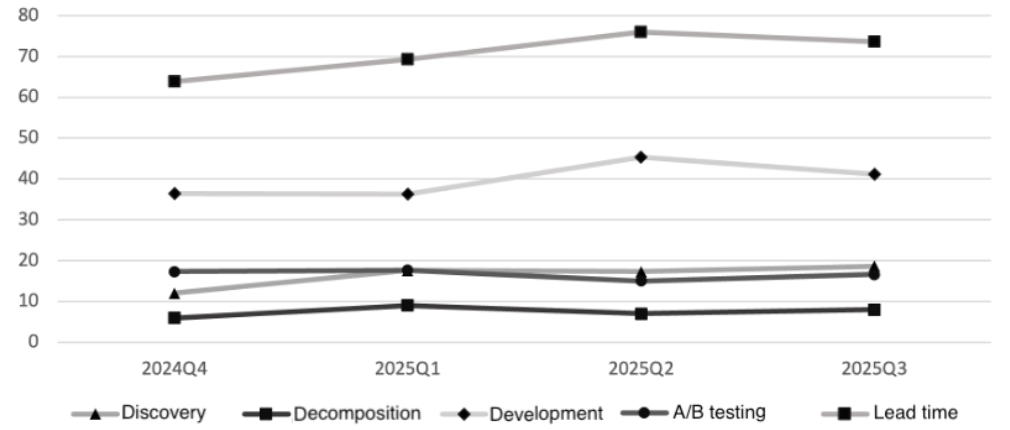
For managerial interpretation, it is important to understand that an increase in the 85th percentile does not always mean a degradation of productivity. Sometimes this reflects a temporary transition period, for example, the introduction of new tools or changes in the team composition. However, if the increase persists for several quarters, this is a sign of a structural problem. In our case, the analysis indicates that improving stability should focus on early stages: decomposition and refinement of requirements. More thorough Discovery before development can reduce variability at the main stage and, consequently, reduce overall lead time.
Thus, quarterly analysis and percentile analysis allow not only to see how metrics change, but also the trajectory of the process. It helps distinguish short-term fluctuations from stable trends, understand where the upper cycle boundary is formed, and what managerial decisions influence it.
Cumulative Flow Diagram (CFD). After analyzing quarterly metrics and percentiles, we move to examining the cumulative flow diagram (CFD). This tool helps evaluate the process holistically: through separate statistical indicators and through the continuity of the flow and balance between stages.
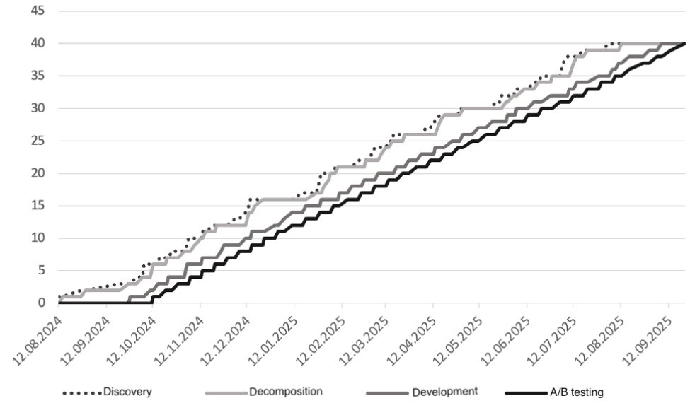
The task at this stage is to track how steadily the team manages the flow of tasks through the system and determine where accumulations or delays occur. The top line on the CFD (lead time) shows how many tasks leave the system; the lower lines reflect how many tasks are in progress and how distribution between stages changes.
Comparing several CFD diagrams across different periods makes it possible to see how the process reacts to managerial decisions, for example, introducing WIP limits, changes in prioritization policy, or adjustments in readiness criteria. For generating a CFD, tasks are distributed by stages (Discovery, decomposition, development, A/B testing) and displayed as cumulative totals. The vertical axis reflects the number of tasks, while the horizontal axis shows time. The distance between lines of different stages represents the amount of work-in-progress (WIP). If the distance between lines increases, this is a signal of task accumulation; if it remains stable, it is an indicator of a healthy flow.
In Figure 4, all lines rise evenly and maintain approximately the same distance between each other. This indicates balanced team workload and stable passage of tasks through the process. The absence of widening intervals between stages shows that new tasks enter the system at the same pace as completed ones leave it. This type of CFD indicates balance between incoming and outgoing tasks, an important sign of a mature flow.
If, however, the distance between lines increases in one area, the diagram allows identifying where bottlenecks occur. For example, if the “Development” line rises more steeply than others, this means that WIP is accumulating at that stage, which indicates overload and the need to revise limits or readiness criteria, which over time would lead to an increase in lead time. In this case, the team could reconsider WIP limits, redistribute tasks, or perform a root-cause analysis of the delays.
The cumulative flow diagram also clearly demonstrates the operation of Little’s Law, which establishes the relationship between the average number of tasks in the system (WIP), throughput, and lead time:
L = λ × W,
where L is the average cycle time, λ is the average processing speed, and W is the average number of tasks in progress [9].
In practice, this means that the stability of lines on the CFD is a visual manifestation of the balance between these parameters. If the flow is uniform, Little’s Law is fulfilled: an increase in the number of tasks in progress immediately reflects in an increase in cycle time, and vice versa. Therefore, CFD is not merely a visualization, but an instrument for verifying whether this balance is maintained.
In our case, the uniform growth of the lines and the absence of noticeable divergence between them indicate stable team productivity. This confirms that current WIP limits are effective and the process functions without accumulating excess work in progress. Thus, CFD analysis allows not only to evaluate the current state but also to quantitatively confirm the stability of the system, which makes this metric key in regular monitoring of flow maturity.
Detailed task-level analysis. After analyzing aggregate metrics and process dynamics, the next step is a detailed examination of individual tasks that fall beyond the 85th percentile. Such analysis makes it possible to move from averaged statistical indicators to concrete cases and identify the real reasons behind increased task duration.
The goal of this stage is to determine which factors lead to deviations: unclear requirements, repeated reviews, priority changes, external dependencies, or technical complexity. Unlike percentiles or CFD, where attention is focused on flow characteristics, here we analyze individual elements that form the “tail” of the distribution and directly influence the upper boundary of lead time.
For analysis, a table with the detailed time spent by tasks in each status is used (Table 1). Comparing stage durations allows determining at which specific step delays occur. As the table shows, Task 1 significantly exceeds the others in the time spent in development: 84 days versus the median values of around 20 to 40 days. Such deviation cannot be explained by randomness and requires separate investigation. Checking indicates that prolonged time in development is often associated with insufficient Discovery or insufficiently refined readiness criteria during intake. Therefore, improving preliminary decomposition and readiness criteria can reduce the likelihood of such cases.
| Task | Discovery | Decomposition | Development | A/B testing | Lead time |
|---|---|---|---|---|---|
| Task 1 | 9 | 2 | 84 | 15 | 110 |
| Task 2 | 12 | 3 | 42 | 10 | 67 |
| Task 3 | 12 | 6 | 19 | 13 | 52 |
| … | |||||
| Task N | 19 | 8 | 26 | 15 | 68 |
Besides individual deviations, it is useful to look for recurring patterns. If several tasks are systematically delayed at the same stage, this may indicate a structural issue: developer overload, lack of expertise, inefficient handoffs between stages, or unsuccessful WIP-organization. Corrective actions are used in such cases, for example, rebalancing the workload, tightening readiness criteria, adding automated checks, or revising prioritization policy.
Detailed task-level analysis also performs a feedback function for the team. It shows how local events affect overall stability and which concrete steps lead to reduction of long cycles. Regular execution of such analysis helps identify recurring causes of delays and gradually eliminate them, thereby reducing the share of tasks falling beyond the 85th percentile and improving delivery predictability.
4.3. Results and Managerial Effects
Regular application of the methodological approach ensures:
- improved accuracy of delivery forecasts through the use of the 85th percentile as a realistic service-level measure;
- stabilization of cycle duration and reduction of the share of tasks that exceed forecast boundaries;
- increased process transparency and strengthened quality of managerial decisions;
- development of a data-driven analysis culture and conscious flow management.
Using statistically grounded metrics allows transitioning from reactive to predictable control of development processes, which is an important element of Kanban-system maturity and contributes to increasing team productivity.
It is important to note that the process of metric analysis should not be one-time. It is part of the culture of continuous improvement, where data tracking and corrective action become a regular team practice. To ensure such sustainability, it is critical that metric collection and updates occur automatically and integrate into the existing task management system without requiring manual activity. This allows maintaining information relevance and using data for operational managerial decisions.
5. Conclusion
The conducted study made it possible to develop and test a methodological approach to designing team effectiveness metrics in IT companies, based on the principles of flow management and statistical analysis of the production cycle. Unlike traditional KPI models focused primarily on output indicators, the proposed approach evaluates effectiveness through the transparency and predictability of task flow, which ensures alignment between operational processes and the strategic goals of the organization.
The methodology, built on the use of cycle-time metrics (lead time), work-in-progress volume (WIP), and team throughput, as well as visualization tools such as the cumulative flow diagram (CFD), makes it possible to transition from subjective assessments to objective quantitative data that characterize the stability and maturity of the production process. Quarterly analysis and stage-level metrics made it possible to identify that the “Development” stage has the greatest impact on overall cycle predictability and forms the upper boundary of lead time. This conclusion is supported by the analysis of aggregated metrics and identification of critical process segments.
Practical recommendations obtained from testing the approach confirm its effectiveness in improving team workflow and increasing the manageability of the development process. The use of median and percentile metrics allows assessing the stability of team work, identifying potential bottlenecks, and coordinating management decisions such as reallocating workload, adjusting readiness criteria, or revising prioritization policy. The cumulative flow diagram, combined with a detailed analysis of time spent in statuses, allows assessing the balance between incoming and completed tasks, confirming the operation of Little’s Law and the maturity of the production rhythm.
Special attention is given to implementing continuous improvement practices based on regular data collection and updating. Consistent monitoring of execution time, workload, and process stability not only helps detect deviations in the early phases but also strengthens the system of operational managerial decision-making. For this, it is advisable to integrate the metric system with corporate analytical tools to automate data collection and reduce manual effort. This helps maintain data relevance and increases the speed of managerial response.
The obtained results demonstrate that the proposed process-oriented approach provides a comprehensive understanding of system behavior and creates a foundation for constructing effectiveness metrics that reflect not only outcomes but also the quality of organizational interaction. It contributes to increasing management transparency, reducing process variability, and strengthening the culture of continuous improvement within teams working under flexible methodologies.
From a scientific point of view, the value of the study lies in the development of a methodological basis for team effectiveness assessment based on flow analysis, as well as in demonstrating the applicability of process-oriented approaches in IT-management. The practical significance is in the possibility of integrating the proposed system of metrics into management dashboards and analytical panels for regular monitoring of flow maturity and supporting managerial decisions.
Further development of the work may include expanding the set of studied indicators, adding metrics for user satisfaction, incorporating technical debt assessment, and adapting the method for multi-command environments in complex organizational structures. This will allow a deeper understanding of the relationships between flow metrics, team dynamics, and strategic stability of digital organizations.
References
- Mil'ner B. Z. 2021. Teoriya organizatsii: uchebnik [Organization Theory: Textbook]. Moscow: Infra-M.
- Chesbro G. and Appel K. 2020. Agile-upravlenie proektami: sovremennye podkhody k effektivnosti komand [Agile Project Management: Modern Approaches to Team Efficiency]. Saint Petersburg: Piter.
- Khekman Dzh. 2018. Komandnaya effektivnost': sozdanie i podderzhanie vysokoeffektivnykh komand [Team Effectiveness: Creating and Maintaining High-Performance Teams]. Moscow: Al'pina Publisher.
- Druker P. F. 2015. Effektivnyy menedzher [The Effective Executive]. Moscow: Vil'yams.
- Anderson D. 2017. Kanban: uspeshnaya evolyutsiya vashego IT-biznesa [Kanban: Successful Evolutionary Change for Your Technology Business]. Moscow: Mann, Ivanov i Ferber.
- Hackman J.R. and Wageman R. 2005. A theory of team coaching. Academy of Management Review, vol. 30, no. 2, pp. 269-287.
- Katzenbach J.R. and Smith D.K. 2018. The Wisdom of Teams: Creating the High-Performance Organization. Boston: Harvard Business School Press.
- Vacanti D. 2018. Actionable Agile Metrics for Predictability. Leanpub.
- Little J.D.C. 1961. A Proof for the Queuing Formula: L = λW. Operations Research, vol. 9, no. 3, pp. 383-387. https://doi.org/10.1287/opre.9.3.383